By using SubsurfaceAI, geoscientists can effectively predict missing well logs without needing to write any Python code, streamlining the integration of ML into traditional G&G workflows.
Everything you need to complete large 2-D and 3-D seismic interpretation projects, >20 times faster than legacy software
Unique solutions to model lamina and outcrop scales heterogeneity and seamlessly integrated with seismic scale reservoir models within one project
Easy-to-use workflows for integrating seismic inversions, well data and make reservoir property grids and maps
Fast interpretation of core photos to deliver “ground-truth” logs of litho-facies, Vshale, porosity and permeability.
Interactively calculation of seismic attributes with data conditioning, seamless integration with well data and reservoir modeling
Advanced 4-D visualization and SRV estimation within fracking stage, evaluate parent-child relations in horizontal drilling
Full-cycle workflow solution for CO2 storage site selection, reservoir mapping and characterization, modeling and leakage monitoring
Build local rock physics templates (RPT) for fast QI interpretation of seismic inversion volumes
Fit-for-purse ML workflows built for integrating production data and near-wellbore seismic attributes for predicting sweet spots and future production
Phone numbers of subsurfaceAI support teams. Request for more information from us
Published case studies listed by products
Recommend hardware, operating systems & cloud
Published case studies listed by reservoir types
Training topics and schedule
List of published technical references and case studies
Well logs are critical for understanding reservoirs and optimizing exploration and production planning. Unfortunately, many wells lack a full set of log curves necessary for quantitative analysis. For example, shear wave sonic logs are often unavailable, and wells drilled 30 years ago might not have conventional sonic logs needed for generating synthetic seismic data for well ties. However, some common logs, like gamma ray and neutron porosity logs, are usually available.
Since well logs reflect the near-wellbore properties of sedimentary rocks, it is reasonable to expect relationships among these logs, even if those relationships are complex and nonlinear. Machine learning (ML) algorithms, such as neural networks and gradient boosting, can model these complex relationships to reconstruct missing well logs. Once trained and validated, these models can be applied to hundreds or thousands of wells in the same basin with a few clicks.
Traditionally, ML work requires Python coding skills. However, SubsurfaceAI allows geoscientists to leverage advanced ML workflows without writing any code. SubsurfaceAI provides user-friendly tools for geoscience and geophysical (G&G) workflows. This blog outlines an ML workflow for predicting missing well logs using available log curves.
In the example project, we have multiple wells in a study area where only one well has a shear sonic log, some have compression wave sonic logs, and all have neutron and gamma ray logs. The goal is to predict shear and compression sonic logs for all wells. The same workflow can also predict other properties like porosity and permeability.
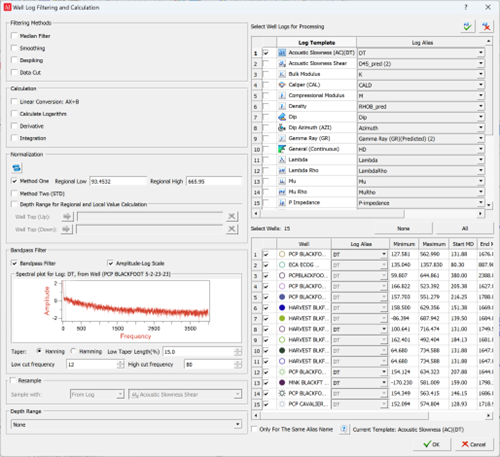
Data conditioning is crucial for any quantitative analysis, especially predictive workflows. SubsurfaceAI software provides tools to remove noise and spikes, normalize logs, resample data, and perform calculations across wells (Figure 1).
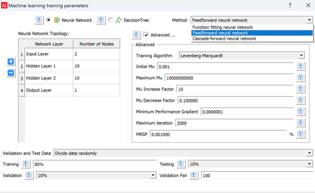
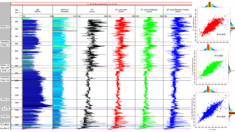
Select wells for training and exclude a few for blind testing. In this study, we use the well PCP 5-2-23-23 in the Blackfoot area of Western Canadian basin for training. Gamma ray, neutron porosity, and sonic logs are used to train three ML models: a feedforward neural network, XGBoost, and Random Forest (Figure 2). Predictions from these models are shown in Figure 3. The training uses 80% of the data, with 10% for validation and 10% for testing. The Random Forest model had the best correlation with the actual sonic log used in training (0.926).
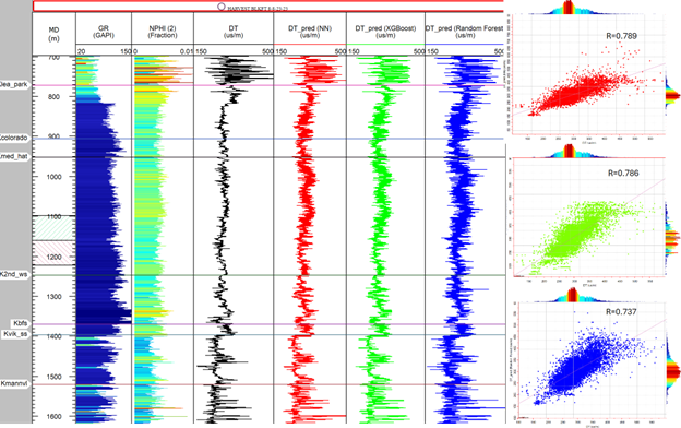
ML models must be validated with data not included in the training set. We used the well Harvest 8-8-23-23 for blind testing. Figure 4 shows the correlation between actual and predicted sonic logs using the three ML models. The correlation in the blind testing well is not as high as in the training well, emphasizing the need for model validation.
After validation, the trained model can be applied to many other wells. For wells drilled decades ago without sonic logs but with gamma and neutron porosity logs, the trained model can predict the missing sonic logs. These predictions can be used to generate synthetic seismograms for better well ties or quantitative seismic interpretation.
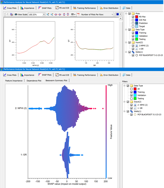
ML models are often seen as “black boxes.” However, tools like Shapley plots, Partial Dependence (PD) plots, and Individual Conditional Expectation (ICE) plots help make ML models more explainable. SubsurfaceAI provides a “Performance Window” to analyze ML models using these tools, helping users understand the relative importance of each input and well to the ML results (Figure 5).
By using SubsurfaceAI, geoscientists can effectively predict missing well logs without needing to write any Python code, streamlining the integration of ML into traditional G&G workflows.
This website uses cookies so that we can provide you with the best user experience possible. Cookie information is stored in your browser and performs functions such as recognising you when you return to our website and helping our team to understand which sections of the website you find most interesting and useful.
Strictly Necessary Cookie should be enabled at all times so that we can save your preferences for cookie settings.
If you disable this cookie, we will not be able to save your preferences. This means that every time you visit this website you will need to enable or disable cookies again.
This website uses Google Analytics to collect anonymous information such as the number of visitors to the site, and the most popular pages.
Keeping this cookie enabled helps us to improve our website.
Please enable Strictly Necessary Cookies first so that we can save your preferences!
