Abstract
In the first two parts of this series, we introduced the motivation and methods behind rule-based reservoir modeling. Part 1 presented the core philosophy—representing geological heterogeneity that controls fluid flow—while Part 2 described how ReservoirStudio (RS) implements those rules to generate geologically consistent 3D models that honor depositional processes.
In this third part, we explore how these concepts perform under dynamic simulation. Using a real-world study from Aker BP ASA in Norway, we compare traditional proportional-layer models (e.g., Petrel-type grids) against rule-based models built in ReservoirStudio that explicitly capture thin mud-drape layers and sub-seismic scale stratigraphic layer patterns in point-bar reservoirs. The results demonstrate dramatic differences in predicted flow behavior, recovery efficiency, and connectivity—proving that the heterogeneity captured by rule-based modeling is not merely visual but fundamentally changes the dynamic response of the reservoir as much as 25% in terms of oil recovery.
Introduction
Reservoir modeling has always balanced two competing priorities: geological realism and simulation efficiency. Traditional static models, with their layer-cake architecture and layer patterns based on few simple rules, often smooth out the fine-scale heterogeneities that actually control flow. Rule-based modeling challenges this simplification by embedding geological process logic directly into the layer construction.
In Part 1, we discussed why capturing rule-based structures—such as shale drapes, erosional truncations, and lateral accretion surfaces—matters for fluid flow. Part 2 described how tools like ReservoirStudio generate such architectures by applying geologic rules instead of geometric interpolation when building the layer model.
Now, in Part 3, we move from theory to practice. Aker BP specialists used ReservoirStudio to construct rule-based point-bar reservoir models with explicit shale drapes. These models were compared to traditional proportional-layer models in a dynamic simulation study. The differences in connectivity, sweep efficiency, and recovery factor were striking.
Modeling Context: Point-Bar Reservoirs and Shale Drapes
Fluvial reservoirs commonly consist of point-bar sand bodies deposited by meandering rivers. Within these sands, thin mud drapes— decimeter – to 1 meter-scale shale layers—develop along lateral accretion surfaces. While often below seismic resolution, these drapes can critically compartmentalize the reservoir, influencing pressure communication and waterflood behavior.
Traditional static modeling systems, such as Petrel, struggle to capture these features. Their vertical layering schemes are usually proportional (or follow-top, follow-bottom) to stratigraphic thickness, meaning the impact of these thin-bed mud layers are not captured or are averaged out. Rule-based modeling, in contrast, defines each depositional element—bar, channel, levee, shale drape—as independent layers governed by geologic rules.
Aker BP sought to test whether maintaining these small-scale heterogeneities in the model would lead to measurable differences in flow response during simulation for a point reservoir. The special concern is forecasted production profiles.
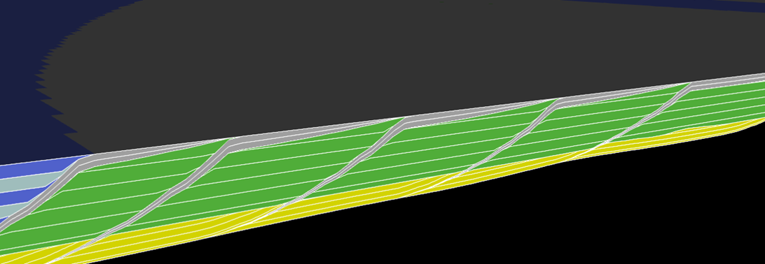
Figure 1. Conceptual point-bar architecture with mud-drape layers generated in ReservoirStudio. Thin shale laminations act as local flow barriers within lateral accretion packages.
Building the Fine-Grid Model in ReservoirStudio
The fine-grid reference model was constructed in ReservoirStudio at sub-meter resolution to explicitly represent thin mud drapes and internal bedding geometry. The depositional rules automatically placed shale layers at accretion boundaries, preserving realistic curvature and continuity.
Each point-bar element consisted of alternating high-permeability sand laminae and low-permeability shale partings. The resulting model reproduced the realistic zig-zag architecture of bar migration, something unattainable in standard layer-cake frameworks.
This fine grid served as the “truth” model for later upscaling and simulation comparisons.
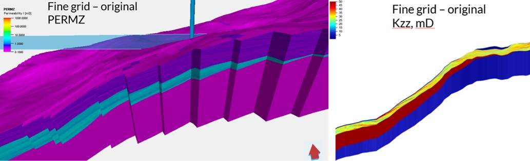
Figure 2. Fine-grid ReservoirStudio model showing explicit shale drapes along lateral accretion surfaces. High-permeability sand (yellow) and low-permeability shale (blue) alternate in realistic geometries.
Upscaling and Simulation Model Preparation
Because the fine grid contained extremely thin layers, direct simulation would be computationally expensive. Therefore, Aker BP generated several upscaled grid versions, each coarsened to different degrees but following the same stratigraphy.
The key upscaled grids included:
- S5: proportional-layer grid with 1 m vertical resolution, same lateral resolution as fine grid.
- S9: proportional-layer grid with 1 m vertical resolution but coarser lateral resolution (2:1).
- S10–S13: rule-based upscaled grids that preserved thin mud layers explicitly during upscaling.
All grids were converted for ECLIPSE simulation through Petrel, ensuring consistent boundary conditions and PVT properties.
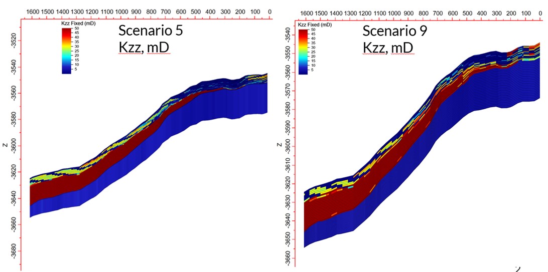
Figure 3. 3D comparison of the fine-grid model and upscaled scenarios S5 and S9 used for testing.
Permeability and Property Assignment
The study considered multiple permeability scenarios. For each grid, PERMX, PERMY, and PERMZ distributions were generated using different upscaling methods:
- Original: Directly from the ReservoirStudio model (geologically consistent).
- Kz 0.1: Same as original but with vertical permeability reduced by factor 0.1 to mimic anisotropy.
- PetrelProxi: Averaged horizontal permeabilities (flat) and PERMZ = PERMX × 0.1, representing a purely numerical approximation.
Additionally, SATNUM regions were defined according to permeability thresholds:
- PERMX < 10 mD → SATNUM = 1
- 10 < PERMX < 100 mD → SATNUM = 2
- PERMX > 100 mD → SATNUM = 3
A single PVT region was used (PVT_2_Seg1_H2) to represent the fluid system for the H2 sand. Initial water saturation (Sw) and pressure were assigned based on J-function relationships.
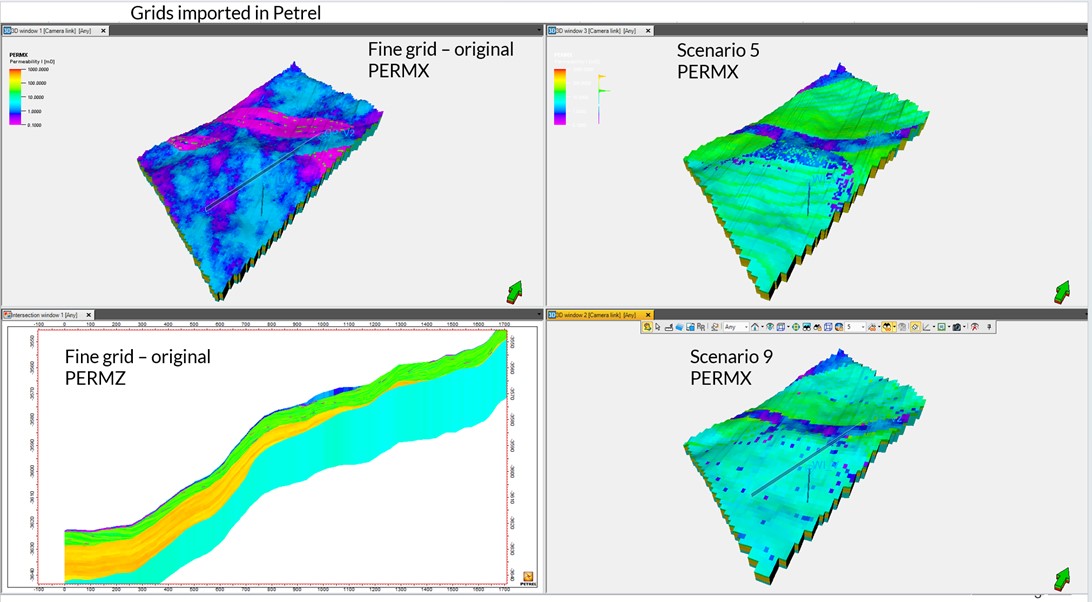
Figure 4. Maps of PERMX and PERMZ for fine grid, S5, and S9 models, showing the effect of vertical upscaling on anisotropy
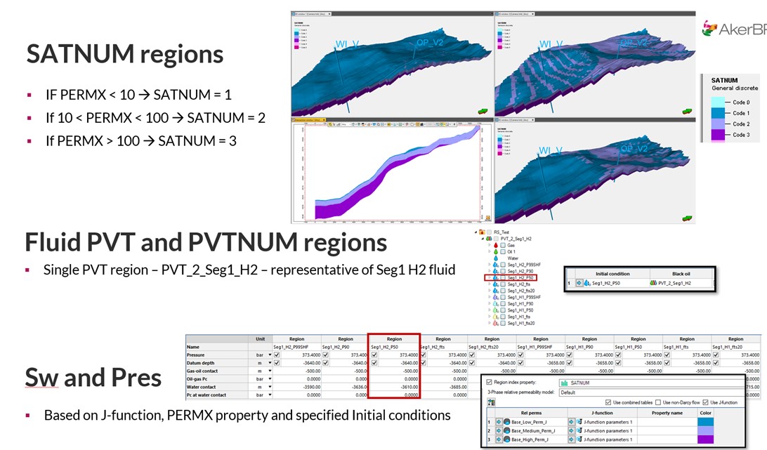
Figure 5. Definition of SATNUM and PVT regions derived from permeability thresholds and J-function mapping.
Flow-Based Upscaling and Volumetric Sensitivity
Upscaling changes both grid geometry and flow properties. To test sensitivity, Aker BP performed flow-based upscaling in Petrel, comparing permeability and saturation transfer from the fine grid to the coarser S5 and S9 grids.
Key parameters screened included:
- PERMX and PERMZ, to evaluate anisotropy preservation.
- ACTNUM, to verify active-cell representation in both high- and low-permeability zones.
This sensitivity analysis highlighted that simple arithmetic averaging (as in PetrelProxi) leads to significant loss of connectivity control, especially in low-permeability mud-drape intervals.
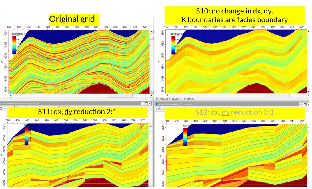
Figure 6. Setup of flow-based upscaling tests comparing fine grid and coarser grids S5 and S9 using Petrel flow-based algorithms.
Dynamic Simulation Scenarios
Dynamic testing focused on three primary cases:
- Fine Grid (FG): the detailed ReservoirStudio model.
- S5 Grid: 1 m thick proportional layers (traditional model).
- S9 Grid: coarser proportional model with 2:1 lateral coarsening.
Each simulation used the same well configuration and fluid model. Oil was produced through a central producer, with flank injectors providing water drive.
The simulation engineer ran multiple scenarios using ECLIPSE, tracking produced-oil rates, cumulative oil, and remaining oil.
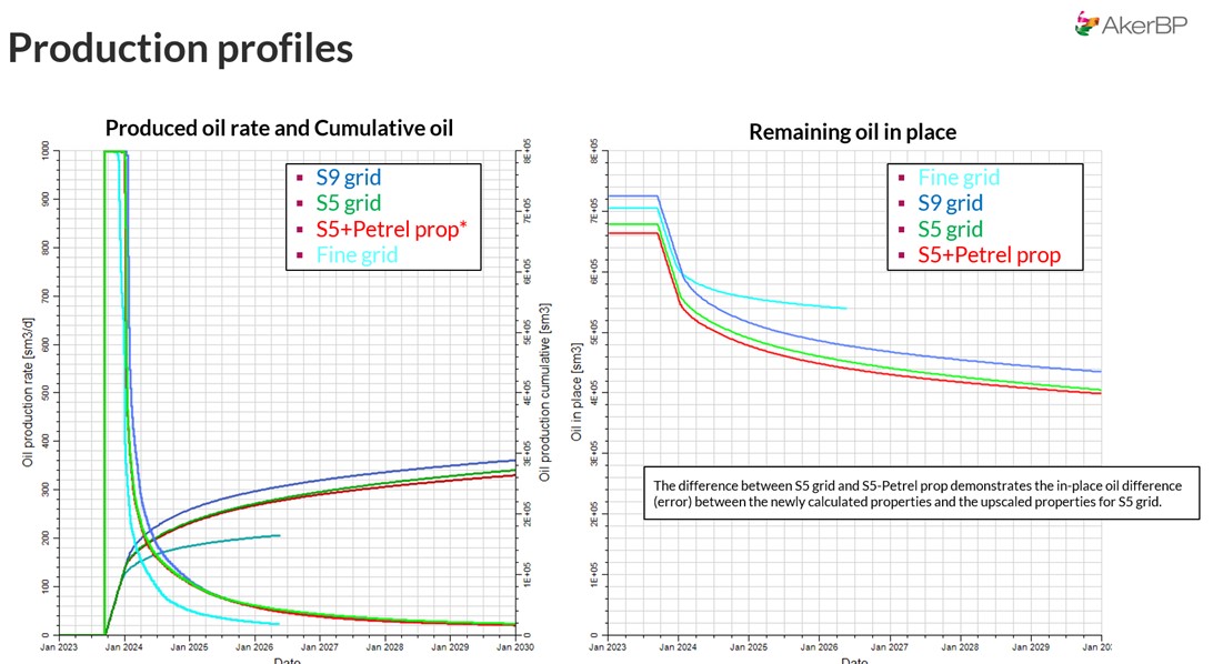
Figure 7. Produced-oil rate and cumulative-oil curves comparing fine grid, S5, and S9 models. The rule-based fine grid predicts slower, more realistic oil recovery than the over-connected proportional grids.
Connectivity Analysis and Saturation Evolution
To understand the dynamic behavior, saturation maps for oil, gas, and water were compared across time steps.
In the fine-grid model, mud drapes restricted vertical communication, creating realistic zones of isolated oil. The high-permeability (sand) zones flooded efficiently, while low-permeability (mud-drape) zones retained oil.
In contrast, the S5 and S9 grids—especially the PetrelProxi versions—showed unrealistically high vertical connectivity. Waterflood fronts advanced too quickly, and recovery factors were significantly over-predicted.
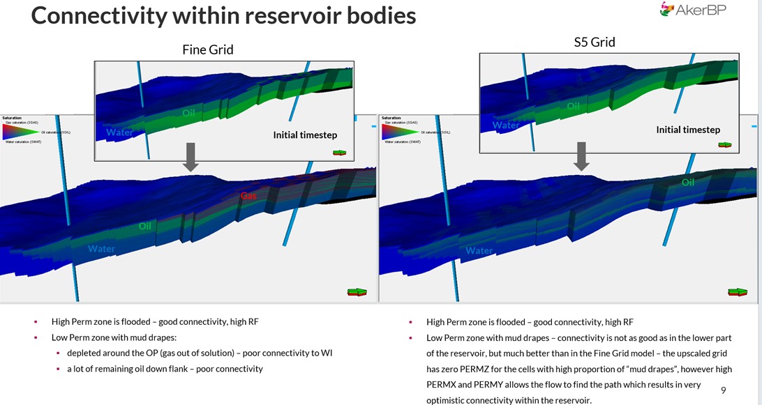
Figure 8. Connectivity comparison between fine-grid, S5, and S9 models. The fine-grid model shows localized depletion and isolated oil pockets, whereas the coarser proportional models flood the entire reservoir unrealistically
Waterflood Behavior and Sweep Efficiency
The fine-grid model revealed distinct flow barriers where oil was trapped beneath mud drapes. Gas evolved locally from solution, forming isolated caps that affected pressure response—behaviors entirely absent in the upscaled proportional models.
In the S5 model, the high-perm zone flooded quickly, but mud-drape barriers were smeared out, leading to artificial crossflow and excessive oil recovery. The difference in cumulative production between fine-grid and S5 Petrel upscaled models illustrated how volumetric “error” directly translates to flow-simulation error.
Dynamic Results for Explicit-Mud Upscaling Cases (S10 – S13)
Recognizing the shortcomings of proportional upscaling, Aker BP generated additional rule-preserving upscaled grids (S10–S13):
- S10: same lateral resolution as fine grid (dx, dy unchanged), explicit mud layers preserved.
- S11: lateral coarsening 2:1, still explicit mud layers.
- S12: coarsening 3:1 (lateral), explicit mud layers; resulted in ECLIPSE solver error due to domain limits.
- S13: same dx, dy as fine grid, but vertically proportional layers (0.2 m).
These models retained the thin-bed connectivity control by explicitly preserving low-permeability mud layers, ensuring realistic flow partitioning even after upscaling.
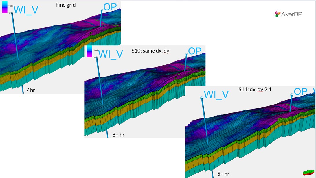
Figure 9. Grid comparison and solver configuration for rule-preserving upscaling cases S10–S13 .
Comparative Simulation Performance
Simulation run-time decreased from roughly 7 hours for the fine-grid case to 5 hours for S11, a reasonable computational saving without major accuracy loss.
More importantly, S10 and S11 reproduced dynamic results nearly identical to the fine grid. Pressure response, oil-rate decline, and cumulative recovery closely matched, proving that preserving explicit mud-layer heterogeneity during upscaling maintains the essential flow physics.
By contrast, proportional models S5 and S9 displayed significantly earlier water breakthrough and 15–25 % higher apparent recovery, an unrealistic outcome when compared to fine-grid truth.
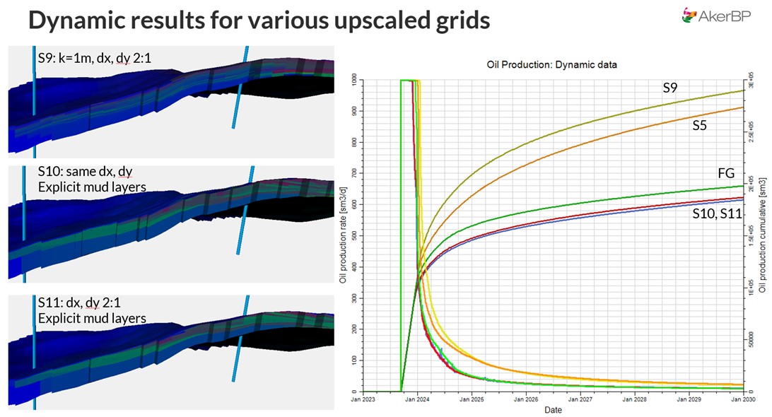
Figure 10. Dynamic simulation comparison for fine grid, S10, and S11 explicit-mud models. Rule-based upscaling achieves nearly identical recovery to fine grid at much lower computational cost.
Why Rule-Based Upscaling Works
Traditional upscaling treats heterogeneity purely numerically: values are averaged vertically or arithmetically. This removes the geological rules that define where barriers exist.
Rule-based upscaling, as implemented in ReservoirStudio, preserves these relationships because each layer or object carries semantic meaning. For instance:
- A “mud drape” layer always acts as a barrier, even when geometrically thinned.
- The lateral continuity of drapes across point-bar surfaces is maintained, preventing artificial vertical leakage.
- During property upscaling, flow-direction biasing ensures permeability tensors retain their anisotropy.
The result is a model that remains geologically and dynamically consistent across scales.
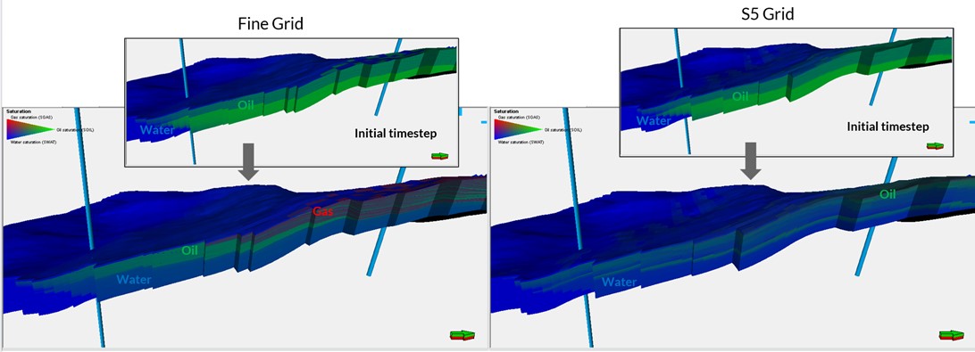
Figure 11. Visualization of simulated flow paths and remaining-oil zones. Models preserving mud drapes (RS S10/S11) show compartmentalized flow and realistic unswept zones, unlike proportional models.
Lessons Learned and Practical Recommendations
The Aker BP study offers several lessons for reservoir modelers seeking to balance accuracy and computational efficiency.
12.1 Preserve Geological Barriers
Even decimeter-scale mud drapes can exert strong control on vertical communication. Ignoring them leads to optimistic recovery forecasts.
12.2 Use Rule-Based Gridding
ReservoirStudio’s rule framework embeds geological logic directly into the grid. Features such as inclined heterolithic stratification and shale drapes can be preserved during coarsening.
12.3 Adopt Flow-Based Property Upscaling
Simple arithmetic or geometric averaging ignores flow directionality. Flow-based upscaling methods better capture anisotropy and transmissibility.
12.4 Balance Resolution with Runtime
Cases S10 and S11 achieved near-fine-grid accuracy at less than 70 % of computational cost. Intelligent upscaling yields efficient yet realistic models.
12.5 Integrate Static–Dynamic Iteration
Rule-based models allow rapid feedback between geology and simulation. Dynamic results can be used to refine depositional rules, improving predictive power.
Broader Implications for Reservoir Management
This study has broader implications beyond the H2 sand case. Many North Sea and Western Canadian fluvial reservoirs share similar point-bar architectures. Recovery optimization in such systems requires accurate prediction of connectivity and compartmentalization.
By embedding geological rules, ReservoirStudio bridges the scale gap between core-scale heterogeneity and reservoir-scale simulation. This is analogous to what SBED accomplished two decades ago at sub-centimeter scales, but now extended to the full 3D reservoir model.
Integration with modern AI frameworks—such as SubsurfaceAI’s CoreAI for core-photo interpretation and IntegrationAI for linking well and seismic data—can further automate rule extraction and model generation. Together, these technologies offer a path toward fully data-driven, geologically sound reservoir modeling.
Conclusions
Dynamic testing by Aker BP conclusively shows that rule-based reservoir models provide more realistic predictions of fluid flow than traditional proportional-layer models.
Key conclusions include:
- Preserving thin mud drapes dramatically alters predicted connectivity and recovery.
- Traditional models over-connect flow units and over-predict oil recovery by 15–25 %.
- Rule-based upscaled models (S10/S11) reproduce fine-grid results with greatly reduced computational time.
- Geological rules, not numerical resolution alone, determine the fidelity of dynamic response.
This three-part series demonstrates that rule-based modeling is not an academic curiosity—it is a practical, scalable method for capturing the heterogeneity that matters most to fluid flow.
As subsurface professionals face increasingly complex reservoirs and tighter budgets, the adoption of rule-based workflows like those in ReservoirStudio will be essential for realistic forecasting and effective reservoir management.
Acknowledgments
The dynamic simulation work and high-fidelity models presented in this blog were executed by the dedicated team at Aker BP. We extend our sincere gratitude to Aker BP ASA for their invaluable technical insight, outstanding collaboration, and willingness to share the results of the dynamic testing of the sector model. This comparative study would not have been possible without the dedicated efforts of the Aker BP subsurface modeling and simulation specialists who championed this critical analysis.
